Neural Style Transfer: Briefly explained and implemented in PyTorch.

Brief History and Motivation Behind NST
Neural Style Transfer (NST) is a technique that emerged from the intersection of deep learning and computer vision. It gained significant attention in 2015 when researchers Leon A. Gatys, Alexander S. Ecker, and Matthias Bethge introduced a groundbreaking paper titled “A Neural Algorithm of Artistic Style.” This paper showcased how convolutional neural networks (CNNs), which are typically used for image recognition tasks, could be repurposed to create stunning artistic images by blending the content of one image with the style of another.
You can read the published paper here.
What is Neural Style Transfer
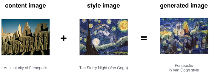
Neural Style Transfer is a deep learning technique that manipulates an image by merging the content of one image with the artistic style of another. Imagine taking a photograph of a cityscape and transforming it to look as if it were painted by Vincent van Gogh or Pablo Picasso. This is achieved by leveraging the power of CNNs to separately extract and recombine the content and style features of images.
The process works by first extracting the content features from the target image and the style features from the reference style image. Through an optimization process, NST adjusts a third image, called the generated image, to minimize the differences in content and style between the target and reference images respectively. The result is an image that maintains the structural integrity of the content image while adopting the stylistic elements of the reference image.

Understanding Content and Style in Images
Definition of Content and Style in the Context of Images
In the context of image processing, “content” and “style” refer to two distinct aspects of an image.
- Content: This pertains to the objects, structures, and the overall layout within an image. For example, in a photograph of a cityscape, the buildings, streets, and skyline represent the content. It captures the essence and the primary subjects of the image.
- Style: Style, on the other hand, encompasses the artistic elements of an image, such as colors, textures, brushstrokes, and patterns. In a painting, the style is what defines the artist’s unique approach, be it the swirling strokes of Van Gogh or the cubist forms of Picasso.
How Humans Perceive Content and Style Differently
We humans have an innate ability to distinguish between content and style when viewing an image. This ability allows us to recognize the same scene (content) even when it is rendered in different artistic styles. For instance, a picture of a tree drawn in a cartoonish manner or painted realistically is still identifiable as a tree. Our brains can separate the structural components (content) from the aesthetic elements (style) seamlessly.
The Role of Convolutional Neural Networks (CNNs) in Distinguishing Content from Style
Convolutional Neural Networks (CNNs) play a pivotal role in the process of Neural Style Transfer by mimicking this human ability to separate content and style. CNNs are a class of deep learning models particularly adept at processing visual data. They are composed of multiple layers that extract features from images in a hierarchical manner.
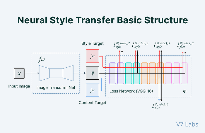
- Content Extraction: In the context of NST, deeper layers of a CNN are used to capture the content of an image. These layers respond to high-level features such as shapes and structures. By using these deeper layers, NST can effectively represent the primary subjects of an image without focusing on fine details.
- Style Extraction: The style of an image is captured using the responses from shallower layers of the CNN. These layers detect lower-level features like edges, textures, and colors. By examining the patterns of activation across these layers, NST can encode the stylistic elements of an image.
The NST process involves optimizing a new image to have similar content representations (from the deeper layers) to the content image and similar style representations (from the shallower layers) to the style image. This optimization is done by minimizing a loss function that quantifies the differences in content and style between the generated image and the target images.

Implementing Neural Style Transfer in PyT🔥rch
Step 1: Install and import required packages
!pip install torch torchvision torch_snippets

# import the required packages
import torch
import torch.nn.functional as F
import torchvision.transforms as T
from torch_snippets import *

# set the device
device = "cuda:0" if torch.cuda.is_available() else "cpu"
print(device)
Step 2: Load and preprocess the images
# Url for the `style image`
!wget https://res.cloudinary.com/ezmonydevcloud/image/upload/v1710325675/turning-pattern.png

# Url for the `content image`
!wget https://res.cloudinary.com/ezmonydevcloud/image/upload/v1710322208/thomas-shelby.jpg
preprocess = T.Compose([
T.ToTensor(),
# we'll use mean and std used for VGG models
T.Normalize(mean=[0.485, 0.456, 0.406], std=[0.229, 0.224, 0.225]),
T.Lambda(lambda x: x.mul_(255))
])
postprocess = T.Compose([
T.Lambda(lambda x: x.mul(1./255)),
T.Normalize(mean=[-0.485/0.229, -0.456/0.224, -0.406/0.225], std=[1/0.229, 1/0.224, 1/0.225]),
])Explanation
- Preprocessing: Prepares the image data to match the distribution of the data used to train the VGG model. This involves normalizing the image tensor to have a specific mean and standard deviation, ensuring consistency in the input data.
- Postprocessing: Reverts the transformations applied during preprocessing, bringing the image data back to its original form or a form suitable for further use, such as visualization.
from PIL import Image
import matplotlib.pyplot as plt

imgs = [Image.open(path).resize((512, 512)).convert('RGB') for path in ['turning-pattern.png', 'thomas-shelby.jpg']]
style_image, content_image = [preprocess(img).to(device)[None] for img in imgs]

# Modify content image with `require_grad=True`
opt_img = content_image.data.clone()
opt_img.requires_grad = True
# Display the images
fig, axes = plt.subplots(nrows=1, ncols=len(imgs), figsize=(len(imgs) * 5, 5))
for idx in range(len(imgs)):
axes[idx].imshow(imgs[idx])
axes[idx].axis('off') # do this, if you want to hide the axis
plt.show()
Step 3: Define the model class, vgg19_modified
from torchvision.models import vgg19, VGG19_Weights

class vgg19_modified(nn.Module):
    def __init__(self):
        super().__init__()
        features = list(vgg19(weights=VGG19_Weights.IMAGENET1K_V1).features)
        self.features = nn.ModuleList(features).eval()

    # Define the forward method, which takes the list of layers and returns the features corresponding to each layer
    def forward(self, x, layers=[]):
        order = np.argsort(layers)
        _results, results = [], []
        for ix, model in enumerate(self.features):
            x = model(x)
            if ix in layers: _results.append(x)
        for o in order: results.append(_results[o])
        return results if layers is not [] else x

# Define the model object
vgg = vgg19_modified().to(device)
This code defines a modified VGG19 model that allows extraction of features from specific layers. By creating a custom vgg19_modified class, it loads the pre-trained VGG19, converts its feature layers to a ModuleList, and enables the forward method to return features from specified layers.
Step 4: Implementing loss functions
Content Loss Function
The content loss function is used to ensure that the generated image retains the primary subjects and structure of the content image. It measures how much the high-level features of the generated image differ from those of the content image.
In practice, this is achieved by passing both the content image and the generated image through a pre-trained Convolutional Neural Network (CNN) and extracting the feature maps from a specific layer. These feature maps represent the high-level content of the images.
The content loss Lcontent is calculated as the mean squared error (MSE) between the feature representations of the content image P and the generated image G:

where:
- Fl is the feature map of the generated image from layer l.
- Pl is the feature map of the content image from layer l.
- i and j index the elements in the feature maps.
This loss function ensures that the generated image G has similar high-level features as the content image P, preserving the overall structure and objects in the scene.
Style Loss Function
The style loss function is designed to capture the stylistic elements of the style image and transfer them to the generated image. It measures how well the textures, colors, and patterns of the style image are replicated in the generated image.
To achieve this, the style of an image is represented using the Gram matrix, which captures the correlations between different feature maps in a layer of the CNN. The Gram matrix Gl for a layer l is defined as:

The style loss Lstyle is calculated as the MSE between the Gram matrices of the style image S and the generated image P:

This loss function ensures that the generated image P replicates the stylistic features of the style image S, including textures and patterns.
Combining Content and Style Losses
In Neural Style Transfer, the total loss function is a weighted sum of the content loss and the style loss:
Ltotal= αLcontent+βLstyle
where:
- α and β are weights that control the relative importance of content and style.
By minimizing this total loss function, the NST algorithm generates an image that balances the structure of the content image with the artistic style of the style image.
Define the gram matrix module
class GramMatrix(nn.Module):
    def forward(self, input):
        b,c,h,w = input.size()
        feat = input.view(b, c, h*w)
        G = feat@feat.transpose(1,2)
        G.div_(h*w)
        return G

# Define the gram matrix's corresponding MSE Loss, GramMSELoss
class GramMSELoss(nn.Module):
    def forward(self, input, target):
        out = F.mse_loss(GramMatrix()(input), target)
        return(out)
Specify the layer that define content loss and style loss
style_layers = [0, 5, 10, 19, 28]
content_layers = [21]
loss_layers = style_layers + content_layers

# Define the loss function for content and style loss values
loss_fns = [GramMSELoss()] * len(style_layers) + [nn.MSELoss()] * len(content_layers)
loss_fns = [loss_fn.to(device) for loss_fn in loss_fns]

# Define the weights associated with content and style loss
style_weights = [1000/n**2 for n in [64,128,256,512,512]]
content_weights = [1]
weights = style_weights + content_weights
We need to manipulate our image such that the style of the target image resembles style_image as much as possible. Hence we compute the style_targets values of style_image by computing GramMatrix of features obtained from a few chosen layers of VGG. Since the overall content should be preserved, we choose the content_layer variable at which we compute the raw features from VGG.
style_targets = [GramMatrix()(A).detach() for A in vgg(style_image, style_layers)]
content_targets = [A.detach() for A in vgg(content_image, content_layers)]
targets = style_targets + content_targets
Step 5: Define optimizer and number of iterations
Even though we could have used Adam or any other optimizer, LBFGS is an optimizer that has been observed to work best in deterministic scenarios. Additionally, since we are dealing with exactly one image, there is nothing random. Many experiments have revealed that LBFGS converges faster and to lower losses in neural transfer settings, so we will use this optimizer
max_iters = 1000
optimizer = optim.LBFGS([opt_img])
log = Report(max_iters)
Step 6: Train the model
Perform the optimization. In deterministic scenarios where we are iterating on the same tensor again and again, we can wrap the optimizer step as a function with zero arguments and repeatedly call it, as shown here.
iters = 0
while iters < max_iters:
    def closure():
        global iters
        iters += 1
        optimizer.zero_grad()
        out = vgg(opt_img, loss_layers)
        layer_losses = [weights[a]*loss_fns[a](A,targets[a]) \
        for a,A in enumerate(out)]
        loss = sum(layer_losses)
        loss.backward()
        log.record(pos=iters, loss=loss, end='\r')
        return loss
    optimizer.step(closure)
# Plot the variation in the loss
log.plot(log=True)
# Plot the image with combination of content and style images
out_img = postprocess(opt_img[0]).permute(1,2,0)
show(out_img)
As you can see our model after the training is successfully able to blend the style with the content of original image. You could try this out on your own images to test it out how it’s performing on those. You could also try out tweaking some parameters or training it for longer iterations, if you are not satisfied with the final result.
You could get the code on my kaggle notebook.
You could also try checking out my other blog posts:
- What is early stopping in deep learning?
- Reinforcement learning 101: Best introduction for beginners
- Genetic algorithm implementation: Code from scratch in Python
See you in future in a different dimension (maybe …)
